Excel INDIRECT Function

The INDIRECT function returns the reference specified by a text string. You can use INDIRECT when you want to change the reference to a cell within a formula without changing the formula itself. You can use this function to create a reference that won't change in case rows or columns are inserted in the worksheet.

Syntax -  INDIRECT(ref_text,a1)

INDIRECT Function Arguments

As shown in the syntax this function has two arguments:

1 - Ref_text : is a reference to a cell that contains an A1-style reference, a R1C1-style reference, a name defined as a reference, or a reference to a cell as a text string.

2 - a1 : TRUE or FALSE.
            - TRUE or ommited, if you are using A1-style reference.
            - FALSE, if ref_text is an R1C1-style reference.

Important: If ref_text refers to another workbook, the other workbook must be open, otherwise INDIRECT returns the #REF! error value.

Using INDIRECT to lock a cell reference

I'll use an example to demonstrate how it works, but using two formulas.

1. In cell A2, type a number (e.g. 500)
2. In cell B5, type this formula:   =INDIRECT("A2")
3. Press the Enter key and the formula will return the content of cell A2. (in this case, will be the number 500)
4. Now on cell B6 type in the formula: =A2 and press Enter. Result will be 500.
5. To confirm that the cell is locked... add a new line at the top of the worksheet.
6. As cell B6 (B5+ 1 added line) uses the INDIRECT function, now returns 0. Formula has locked cell A2!
7. Cell B7(B6+ 1 added line) which contains the link still returns 500 because the formula has changes to A3

Now with a picture:

Cell reference locked with Indirect function

As you can see on the right side, after adding one line the cell reference in the Indirect function remains unchanged.

Indirect within a Vlookup

This can be an explosive combination of excel functions.

Here is one good example. Imagine that you have an excel file with several worksheets where each one of them contain the sales made in different cities. Then you have one more sheet - overview - where you want to be able to visualize sales of a certain city based on your selection.

On cell B4 of the picture above you can type/select the city name (it must match one of the sheets names). In this case I've selected NewYork on cell B4. The formulas used on cell C5 and cell D5 will return the "Total" sales available in the second Sheet of this workbook named "NewYork".

Cell C5  -   =VLOOKUP("Total",NewYork!$A$1:$D$15,2,0)
Formula explained:
1 - Search "Total"
2 - On a sheet named NewYork - Range $A$1:$D$15
3 - Retrieve data from column 2 of the selected range (will return data from collumn B on Sheet      
     NewYork if Total is found on collumn A)
4 - Exact match - 0 

Cell D5  -   =VLOOKUP("Total",INDIRECT("'"&B4&"'!A1:B30"),2,0)
Formula explained:
1 - Search "Total"
2 - On sheet that has a name equal to cell B4 - NewYork and on Range $A$1:$B$30
3 - Retrieve data from column 2 of the selected range (will return data from collumn B on Sheet      
     NewYork if Total is found on collumn A)
4 - Exact match - 0 


Do not forget the single quotes - INDIRECT("'"&B4&"'!A1:B30")

Now, I'll select Toronto instead of NewYork and the result is:

As you can see in this picture, cell C4 remains with the same value while cell D4 has changed to "208". Why ?
When I've changed the city name from NewYork to Toronto, the formula on cell C4 remained unchanged and is still retrieving the Total from Sheet Named "NewYork". But the formula on cell D4, has adapted itself  (INDIRECT("'"&B4&"'!A1:B30")) according the new content of cell B4 and is now retriveing data from Sheet Name Toronto.

Create a Reference To a Different Sheet or Workbook

In case you need to refer to cells on other worksheets INDIRECT formula can help.

Here are some examples:

Refer to cell A4 on a sheet named according to the value on cell A10

1 - Open a new workbook, add a second sheet called Data and a third sheet called Overview
2 - On the first sheet, on cell A10 enter the text Data
3 - On cell D5 on the same worksheet enter this formula: =INDIRECT("'" & A10 & "'!A4")
4 - Press Enter (Case 1)
5 - As a result cell D5 will return the content of cell A4 on worksheet Data
6 - Change the content of cell A5 from Data to Overview and press Enter (Case 2)
7 - The result of cell D5 will now be the content of cell A4 on worksheet Overview

If you delete the content of cell A10 on the first sheet of your workbook, the above mentioned formula will return an error. To prevent this, you can add an IF function:
=IF(A10="","",INDIRECT("'" & A10 & "'!A4"))


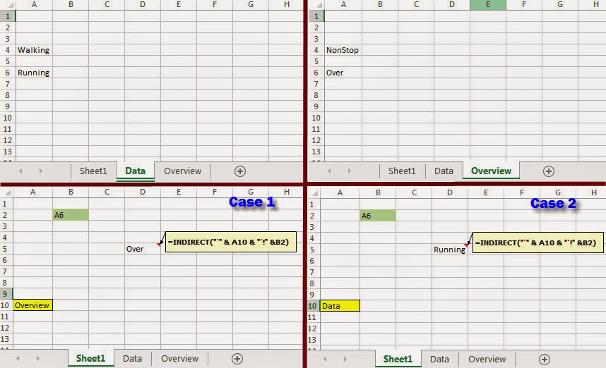
Refer to a the Cell mentioned in cell B2 value on a sheet named as the value on cell A10

In this example both the reference cell as well as the worksheet name are available in two diferent cells of your current worksheet.

The formula that you should use is:  =INDIRECT("'" & A10 & "'!" & B2)

Cell A10 contains the worksheet number and cell B2 contains the cell address that you want to refer to.

If you delete the content of cell A10 or B2 on the first sheet of your workbook, the above mentioned formula will return an error. To prevent this, you can add an IF function:
=IF(OR(A10="",B2=""),"",INDIRECT("'" & A10 & "'!" & B2))